This post is about estimating the parameter of a Bernoulli distribution from observations, in the “Dempster” or “Dempster–Shafer” way, which is a generalization of Bayesian inference. I’ll recall what this approach is about, and describe a Gibbs sampler to perform the computation. Intriguingly the associated Markov chain happens to be equivalent to the so-called “donkey walk” (not this one), as pointed out by Guanyang Wang and Persi Diaconis.
Denote the observations, or “coin flips”, by 


In a Bayesian approach, we would specify a prior distribution on the parameter; for example a Beta prior would lead to a Beta posterior on
Given observations 


How do we obtain the distribution of these sets 
![u\in [0,1]^N](https://s0.wp.com/latex.php?latex=u%5Cin+%5B0%2C1%5D%5EN&bg=FFFFFF&fg=181818&s=0&c=20201002)


From this joint density we can work out the conditionals. We can then express the Gibbs updates in terms of the endpoints of the interval 

- Sampling
.
- Sampling
.
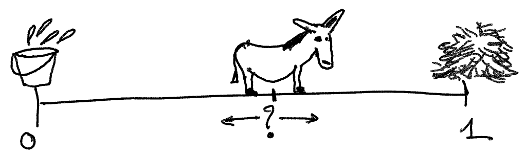
This is exactly the model of Buridan’s donkey in refs [2,3] below. The idea is that the donkey, being both hungry and thirsty but not being able to choose between the water and the hay, takes a step in either direction alternatively.
The donkey walk has been generalized to higher dimensions in [3], and in a sense our Gibbs sampler in [4] is also a generalization to higher dimensions… it’s not clear whether these two generalizations are the same or not. So I’ll leave that discussion for another day.
A few remarks to wrap up.
- It’s a feature of Dempster’s approach that it yields random subsets of parameters rather than singletons as standard Bayesian analysis. Dempster’s approach is a generalization of Bayes: if we specify a standard prior and apply “Dempster’s rule of combination” we retrieve standard Bayes.
- What do we do with these random intervals
, and these proportions are transformed into measures of agreement, disagreement or indeterminacy regarding the set of interest, as opposed to posterior probabilities in standard Bayes.
- Dempster’s estimates depend on the choice of sampling mechanism and associated auxiliary variables, which is topic of many discussions in that literature.
- In a previous post I described an equivalence between the sampling mechanism considered in [1] when there are more than two categories, and the Gumbel-max trick… it seems that the Dempster’s approach has various intriguing connections.
References:
- [1] Arthur P. Dempster, New Methods for Reasoning Towards Posterior Distributions Based on Smple Data, 1966. [link]
- [2] Jordan Stoyanov & Christo Pirinsky, Random motions, classes of ergodic Markov chains and beta distributions, 2000. [link]
- [3] Gérard Letac, Donkey walk and Dirichlet distributions, 2002. [link]
- [4] Pierre E Jacob, Ruobin Gong, Paul T. Edlefsen & Arthur P. Dempster, A Gibbs sampler for a class of random convex polytopes, 2021. [link]

Interesting! Can’t we also view this as a standard partially-collapsed Gibbs sampler on the joint space of both \theta (with a uniform prior on [0, 1]) and the auxiliary variables u? That is, a partially collapsed version of the Gibbs sampler that alternates sampling
1. u in Group 1 and \theta conditional on u in Group 0
2. u in Group 0 and \theta conditional on u in Group 1
The sampler would be partially collapsed because we never actually need to sample anything other than the minimum/maximum u in each group (i.e. we can skip sampling the remaining u’s and we can skip sampling \theta).
Minor correction to my previous comment: The uniform[0,1] prior should be on the auxiliary variables u and not on \theta.
Indeed, the partially-collapsed Gibbs-sampler interpretation shows that you can run the algorithm without selecting a prior for \theta at all! Afterwards, if you need samples from the posterior of \theta, you can pick some prior for \theta and draw samples from it truncated to the intervals spanned by the max/min values of the auxiliary variables in the two groups.
Yes that’s right: you can obtain “random sets” first, without specifying a prior, then sample points within them according to some prior distribution truncated on these sets, and (with an appropriate weighting!!) this will deliver samples from a standard posterior distribution (that corresponds to the prior distribution employed to sample points within the sets). This is a particular application of “Dempster’s rule of combination”. And this is why Dempster-Shafer can be viewed as a generalization of standard Bayes, in my understanding.
Could you explain a bit what’s the role of \theta in your paper? It doesn’t seem to appear here but in your paper there’s an extra step computing it with proposition 3.2 equation (3.4). I thought in the Gibbs sampler you’re only updating u_i|u_-i (because only they’re distributional) so \theta isn’t going to be involved at all. What am I missing?
Also there seem to have no definition for \triangle(\theta)^{N_k} in proposition 3.2. Is there any graphical illustrations that I can understand this proposition and its proof better?
Ok, so maybe what’s proposed in your paper is a different kind of Gibbs sampler than the Donkey, and I right? Because here I’m not seeing any involvement of uniform sampling at all, which seems to be the key in your paper.